Stock Price Forecasting w/ XGBoost

The full Jupyter notebook for this experiment can be found here.

Objective

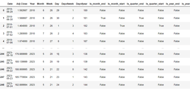
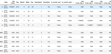
The objective of this experiment is to build and train a model to predict the daily adjusted closing prices of Tesla (TSLA) 1 year into the future. This experiment will consist of data starting from TSLA's IPO date which is 2010-06-29 to 2023-05-24. The data is taken from yahoo finance using a python library called yfinance. After downloading, the dataset looks like this:

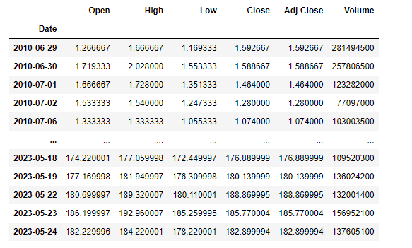
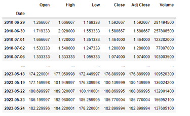
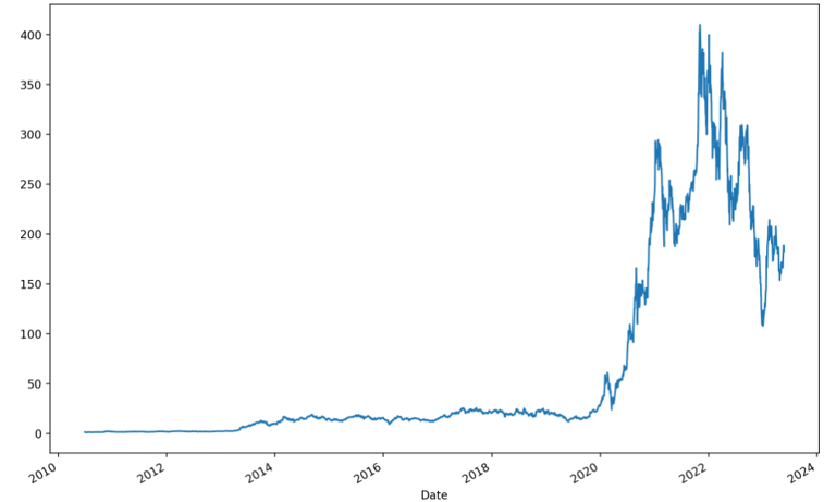
Altogether we have 3249 days of data, excluding the weekends. This plot below shows the adjusted closing price of TSLA’s entire dataset.

In this experiment, I aim to utilize XGBoost to accurately forecast TSLA’s performance in one years time. However, since the data from years 2010 - 2019 are so small compared to the recent years’ data, I will perform time series cross validation to train sectioned date ranges in order to achieve a better trained model.

To evaluate the effectiveness of my model, I will use the root mean square error (RMSE) score where the lower the score, the more accurate the prediction.

Exploratory Data Analysis (EDA)

In order to understand the data set more, I performed some EDA on the dataset. I looked at monthly adjusted closing price, annual adjusted closing price, adjusted closing price for each day of the week. Performing EDA will give me more insight on the data, its growth and its patterns.

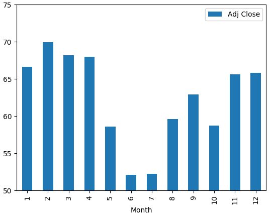
The plot below shows the average adjusted closing price for each month. We can see that mid year months tend to have a lower value.

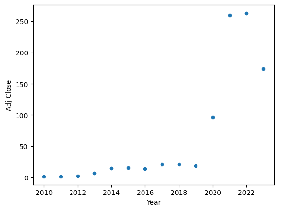
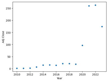
The plot below shows the average adjusted closing price for each year. We can see the growth in 2020 and slight pullback in 2023.

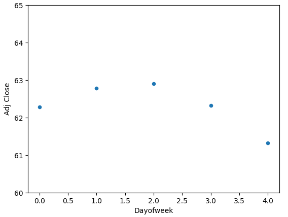
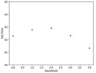
The plot below shows the average adjusted closing price for each day of the week. We can see that the end of the week seems to be slightly lower than the mid week.

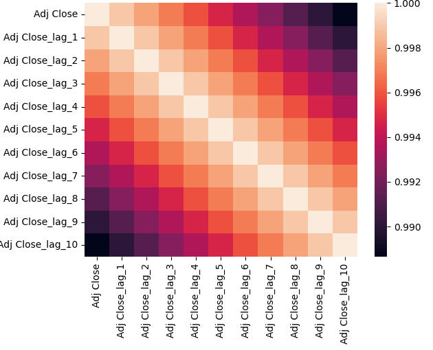
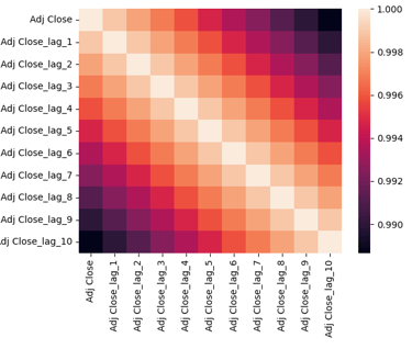
I added some lags to the dataset in order to see the correlation of previous days’ vs the current day. The heatmap below shows the correlation of lags with the Adjusted Close price. As expected, the more recent the price, the more correlated it is.

Feature Engineering

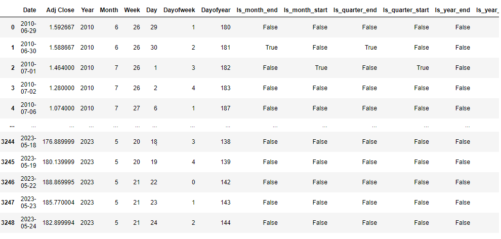
For this project, I decided to create some additional features to improve the accuracy of my model by using the help of fastai. I have added 13 new features for model training. These features include: Year, Month, Week, Day, Dayofweek, Dayofyear, Is_month_end, Is_month_start, Is_quarter_end, Is_quarter_start, Is_year end, and Is_year_start.

After the adding the new features, the dataset looks like this:

Training / Test Split

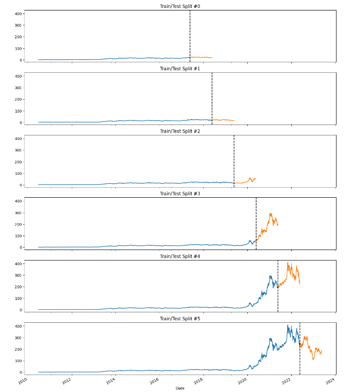
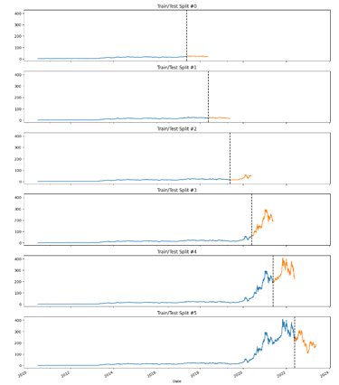
Given the large span of data (13 years), I figured the more accurate way to train/test split would be by Time Series Cross Validation. Scikit learn conveniently has a model that helps split and test data according to your needs. In this experiment, I will split the entire data by 6 for training and the following year for testing. Doing so in chronological order would also prevent information leak in the model.

The code below displays the model creation. The split train / test data will be assigned accordingly. The FEATURES are all the columns of data we wish to train. The added lags could give us a slight boost in accuracy.

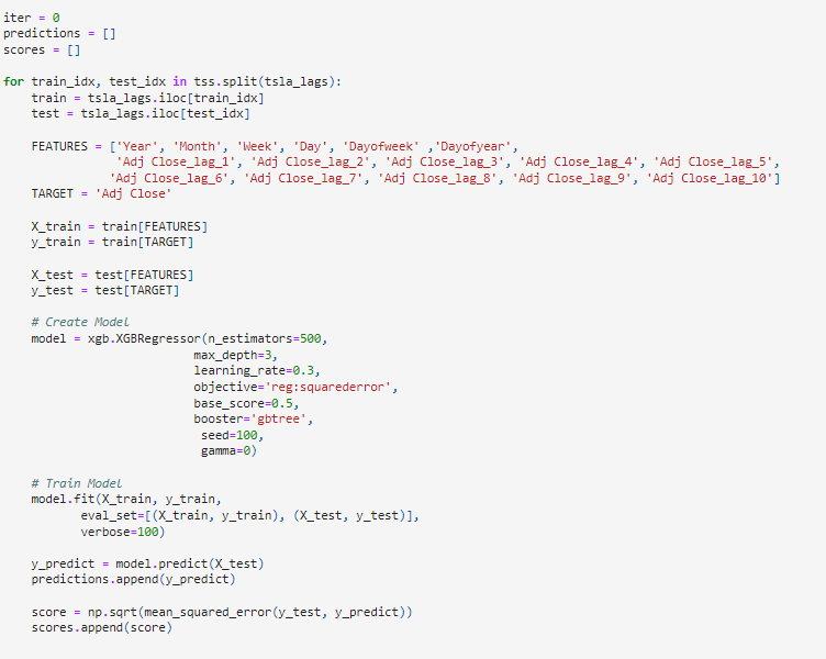
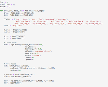
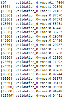
Running this code would display the root mean square error (RMSE). As you can see after about 11000 iterations, the score seems to have stabilized at its minimal.

Predicting the Future

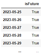
In order to predict TSLA 1 year’s time into the future I had to create a skeleton date frame and combine it to the current data. Since the dataset ends at 05-24-2023, the start of the future dataset will be on 05-25-2023. Note that I also added a new column called [‘isFuture’] to indicate which rows of data are in the past and which is in the future.

After combining the datasets, and re-implementing the feature engineering, the dataset looks like this:

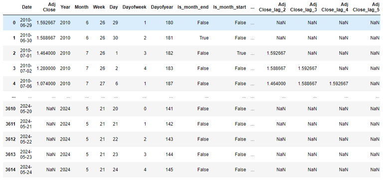
Now all that’s left to do is to retrain all of the data and plot all the rows where [‘isFuture’] is true.

Findings

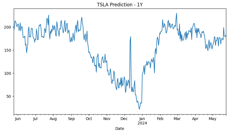
The model has successfully predicted the stock prices in one years time. Though this model is not perfect. In the future I would like to introduce feature scaling to the date lags so that the model could be even more accurate. I would also like to introduce the stocks financials as features that could affect the stock price as well. Lastly, I aim to deploy this into an open sourced website so people could see the forecast for whichever stock they want.

The full Jupyter notebook link for this project can be found here.